Published on: Nov 26, 2021

Color constancy of an image using Chromatic adaptation

Color constancy

Color constancy is the tendency of the human color system that ensures the color perception of objects is relatively constant under varying illumination conditions. It means we observe the same object colors for different light conditions.

Like for example, under a greenish light source, the color of the apple looks relatively red even though the intensity of the green wavelength is greater than other colors. It's unknown how we (and some other animals) have this color perception system.

Several mechanisms like metamerism, chromatic adaptation, memory map, etc. are involved in achieving color constancy. Metamerism happens when two object looks the same color even though the reflectance wavelengths are not the same but overall color is the same. Our memory map of object colors helps our eyes to adjust the color perception after some time under different illuminations.

Color constancy is not true in every object case, for some objects under certain illumination conditions, it could be inverse. Color constancy happens in most of the cases for objects if we have seen them before and for other objects/surfaces, we observe the color of major intensity wavelength. Color constancy depends heavily on the illumination source and neighborhood surface.

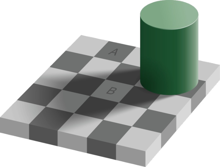Even though both A and B are the same gray color, A appears darker than B because of shadow from the cylinder which changes illumination on B

Several theories like photoreceptor sensitivity, retinex, color map, etc, try to measure the color constancy using different mechanisms.

Chromatic adaptation

Chromatic adaptation is one of the mechanisms involved in color constancy and is defined as the ability of human color perception to adjust the retina/cortex sensitivity for changes in the illuminant color system. Chromatic adaptation is closely related to the adjustment of cone sensitivity that happens in our eyes when the illumination changes. Like our eyes adjust to see the objects as constant colors under different day-light conditions like sunrise, mid-day, and sunset. In all these conditions, we perceive object colors as the same. This could be opposite in some conditions where we see opposite colors instead of relative colors.

In computer vision, computation color constancy is achieving human color constancy using different methods based on color constancy mechanisms. And chromatic adaptation technique is one of the methods to achieve computational color constancy based on illumination.

Von Kries transform

The Von Kries chromatic adaptation technique is based on the LMS cone sensitivity response function. LMS cones responses in the retina are independent of each other and they adjust independently for varying illuminations. Each cone increases or decreases responsiveness based on illuminant spectral energy. Each cone cell gains (increase or decrease) some spectral sensitivity response to adapt for new illumination from the previous illumination to perceive object constant colors.

Based on LMS cones gain, Von Kries adaptation transforms one illuminant to other to keep the white color constant in both systems. Von Kries transform based on LMS cone sensitivity is the base for chromatic adaptation transforms proposed later.

Chromatic adaptation transform

Von Kries chromatic adaptation transformation is a linear transformation of the source color to destination color based on LMS cones gain for adaptation to destination illuminant. That is, we can transform the color in one illuminant to other illuminants if we scale the color with a gain of LMS for adaptation to color constancy.

If you're not familiar with concepts like CIE RGB, CIE XYZ tristimulus values, chromaticity diagram, and other color science topics, please refer to those topics at my previous blog about color-science.

The destination LMS cone responses can be calculated by multiplying the gain LMS with source LMS cone responses. In matrix form, the representation is

where L, M, and S of source and destination are represented in CIE LMS color space, and $L_{D}/L_{S}$, $M_{D}/M_{S}$, and $S_{D}/S_{S}$ are gain factors for source to destination illumination adaptation.

As color representation in LMS color space is difficult and not practiced, transform the LMS color space to CIE XYZ. When a transformation is performed in CIE XYZ or any other space but not LMS cone space is called Wrong Von Kries.

where the transformation matrix $M_{A}$ with dimensions $3x3$ and independent gain control factors $(a, e, i)$ is called chromatic adaptation transform (CAT) matrix. Each CAT model give different CAT matrices for transformation from LMS cone space to CIE XYZ.

Wrong Von Kries transform by XYZ gain scaling to CIE XYZ tristimulus values of the source is,

We can convert CIE XYZ to LMS cone space and then back to CIE XYZ with $M_{A}$, then we can change Wrong Von Kries to general Von Kries as,

The generalized version of Von Kries for CIE XYZ white point reference is,

$(X, Y, Z)$ values for source and destination are illuminant white point values in CEI XYZ.

White point is the color that is formed when all cone sensitivity responses are maximum.

Implementation of Chromatic adaptation transform

We will implement chromatic adaptation for converting source image to destination illuminant by applying CAT. Chromatic adaptation for an image is implemented in two steps

1. Estimate scene illuminant of image
2. Convert source image to destination illuminant with source illuminant obtained in step 1

Illumination estimation of image

Illumination estimation is predicting tristimulus values (CIE XYZ) for the white point of the illuminant light source under which the reference image has been taken. These predicted white point tristimulus values were then later used for CAT. Illumination estimation is a very crucial step in chromatic adaptation. Several illumination estimation methods exist like

• Gray world assumption
• White patch retinex
• Reflection model

The above methods are suitable for uniform illumination, for nonuniform illumination Retinex models are widely used.

For now, we use the Gray world assumption for illumination estimation

Gray world assumption illuminant estimation

Gray world assumption is a simple method that assumes image contains objects with different reflectance colors uniformly from minimum to maximum intensities and averaging all pixel colors gives gray color. Illumination estimation is calculated by averaging all pixel values for each channel. For an image with equal representation of colors, illumination estimation gives average color gray.

where $R_{avg}$, $G_{avg}$, and $B_{avg}$ are means of each image channel (R, B, G). Scale the mean values to the maximum intensity value of an image which is generally 255 (8-bit).

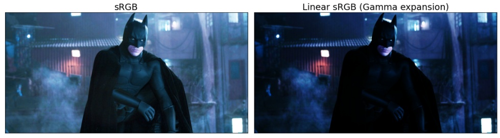
Images are generally stored in JPEG or PNG in sRGB format. To mimic the human perception of non-linear luminance factor, while taking pictures, exposure values are Gamma corrected with a value close to 2.2. And any image processing operation should be applied on linear RGB values by converting sRGB gamma to linear RGB without gamma.

Read source image to which we apply chromatic adaptation and transform to destination illuminant,

1import numpy as np
2import cv2
3
4# read image which generally in sRGB format
5img = cv2.imread('input.jpg')
6# reverse channel order from BGR to RGB
7img = img[:, :, ::-1]
8# scale image in range [0.0, 1.0]
9img = img / 255.0
10

Convert sRGB image to linear RGB

1def srgb_to_linear(srgb):
2    # 'sRGB' in [0.0, 1.0]
3
4    ln_rgb = srgb.copy()
5    mask = ln_rgb > 0.04045
6    ln_rgb[mask] = np.power((ln_rgb[mask] + 0.055) / 1.055, 2.4)
7    ln_rgb[~mask] /= 12.92
8    return ln_rgb
9
10def linear_to_srgb(linear):
11    # 'linear RGB' in [0.0, 1.0]
12
13    srgb = linear.copy()
14    mask = srgb > 0.0031308
15    srgb[mask] = 1.055 * np.power(srgb[mask], 1 / 2.4) - 0.055
16    srgb[~mask] *= 12.92
17    return np.clip(srgb, 0.0, 1.0)
18

Apply gray world on linear RGB image and get illuminant

1def get_gray_world_illuminant(img):
2    # image in sRGB with range [0.0, 1.0]
3    # convert sRGB to linear RGB
4    ln_img = srgb_to_linear(img)
5    # mean of each channel
6    avg_ch = ln_img.mean(axis=(0, 1))
7    # convert back RGB mean values to sRGB
8    return linear_to_srgb(avg_ch)
9

Illuminant for the image is

1illuminant = get_gray_world_illuminant(img)
2

1print(illuminant) => array([0.29078475, 0.39055316, 0.50858647])
2

Illuminant for the above image is [0.29078475, 0.39055316, 0.50858647]. For the output illuminant, we can say that the blue color influence is higher than other color wavelengths in the image.

Now we have the illuminant of the source image, next apply chromatic adaptation for this image.

Chromtic adaptation

We have source illuminant, to transform to destination illuminant, we consider D65 standard illuminant for the destination which is standard for digital images and displays. We assume that the source image was taken under a different illuminant and we now transform that image to D65 illuminant.

Illuminant for D65 white is [0.95047, 1., 1.08883], these are the CIE XYZ values for white point of sRGB D65. sRGB values for D65 white point (all values are 255) is (1.0, 1.0, 1.0) which is destination illuminant white point.

We implement chromatic adaptation transform step-by-step.

Every operation should be applied on linear RGB

First, convert illuminant sRGB values to CIE XYZ.

1RGB_TO_XYZ = np.array([[0.412453, 0.357580, 0.180423],
2                       [0.212671, 0.715160, 0.072169],
3                       [0.019334, 0.119193, 0.950227]])
4
5XYZ_TO_RGB = np.array([[3.240481, -1.537151, -0.498536],
6                       [-0.969256, 1.875990, 0.0415560],
7                       [0.055647, -0.204041, 1.057311]])
8
9def srgb_to_xyz(srgb):
10    # convert 'sRGB' to 'linear RGB'
11    rgb = srgb_to_linear(srgb)
12    # convert 'linear RGB' to 'XYZ'
13    return rgb @ RGB_TO_XYZ.T
14
15def xyz_to_srgb(xyz):
16    # convert 'XYZ' to 'linear RGB'
17    rgb = xyz @ XYZ_TO_RGB.T
18    # convert back 'linear RGB' to 'sRGB'
19    return linear_to_srgb(rgb)
20
21def normalize_xyz(xyz):
22    # normalize xyz with 'y' so that 'y' represents luminance
23    return xyz / xyz[1]
24

Convert sRGB to XYZ passing source and destination white points

1# source illuminant white point obtained from previous step
2src_white_point = illuminant
3# destination illuminant white point scale to 1.0
4dst_white_point = (1.0, 1.0, 1.0)
5
6# convert white point in 'sRGB' to 'XYZ'
7# and normalize 'XYZ' that 'Y' as luminance
8xyz_src = srgb_to_xyz(src_white_point)
9n_xyz_src = normalize_xyz(xyz_src)
10xyz_dst = srgb_to_xyz(dst_white_point)
11n_xyz_dst = normalize_xyz(xyz_dst)
12

Next, convert XYZ values to LMS cone space by transforming XYZ values with CAT transform matrix. Multiple CAT matrices exist and the Bradford model is popular among all these types.

1BRADFORD = np.array([[0.8951, 0.2664, -0.1614],
2                     [-0.7502, 1.7135, 0.0367],
3                     [0.0389, -0.0685, 1.0296]])
4
5VON_KRIES = np.array([[0.40024, 0.70760, -0.08081],
6                      [-0.22630, 1.16532, 0.04570],
7                      [0.00000, 0.00000, 0.91822]])
8
9SHARP = np.array([[1.2694, -0.0988, -0.1706],
10                  [-0.8364, 1.8006, 0.0357],
11                  [0.0297, -0.0315, 1.0018]])
12
13CAT2000 = np.array([[0.7982, 0.3389, -0.1371],
14                    [-0.5918, 1.5512, 0.0406],
15                    [0.0008, 0.2390, 0.9753]])
16
17CAT02 = np.array([[0.7328, 0.4296, -0.1624],
18                  [-0.7036, 1.6975, 0.0061],
19                  [0.0030, 0.0136, 0.9834]])
20

Convert XYZ values to LMS and get gain scale factors by dividing destination LMS with source LMS.

1def get_cat_matrix(cat_type = 'BRADFORD'):
2    if cat_type == 'BRADFORD':
3        return BRADFORD
4    elif cat_type == 'VON_KRIES':
5        return VON_KRIES
6    elif cat_type == 'SHARP':
7        return SHARP
8    elif cat_type == 'CAT2000':
9        return CAT2000
10    else:
11        return CAT02
12
13def xyz_to_lms(xyz, M):
14    return xyz @ M.T
15
16def get_gain(lms_src, lms_dst):
17    return lms_dst / lms_src
18
19def transform_lms(M, gain):
20    return np.linalg.inv(M) @ np.diag(gain) @ M
21

1# get CAT type matrix
2cat_m = get_cat_matrix('BRADFORD')
3
4# convert 'XYZ' to 'LMS'
5lms_src = xyz_to_lms(n_xyz_src, cat_m)
6lms_dst = xyz_to_lms(n_xyz_dst, cat_m)
7# LMS gain by scaling destination with source LMS
8gain = get_gain(lms_src, lms_dst)
9
10# multiply CAT matrix with LMS gain factors
11ca_transform = transform_lms(cat_m, gain)
12

ca_transform() applies chromatic adaptation transformation on LMS gain factors and then converts back the LMS values to XYZ by multiplying with the inverse transform of CAT matrix.

Transform the source image to destination illuminant by multiplying XYZ values with chromatic adaptation transformation XYZ values.

1# convert 'sRGB' source image to 'XYZ'
2src_img_xyz = srgb_to_xyz(img)
3
4# apply CAT transform to image
5transformed_xyz = src_img_xyz @ ca_transform.T
6
7# convert back 'XYZ' to 'sRGB' image
8transformed_img = xyz_to_srgb(transformed_xyz)
9

transformed_img is the final image after transformation.

The final chromatic adaptation function that transforms source image to destination illuminant is

1def chromatic_adaptation_image(src_white_point, dst_white_point, src_img, cat_type = 'BRADFORD'):
2    # convert white point in 'sRGB' to 'XYZ'
3    # and normalize 'XYZ' that 'Y' as luminance
4    xyz_src = srgb_to_xyz(src_white_point)
5    n_xyz_src = normalize_xyz(xyz_src)
6    xyz_dst = srgb_to_xyz(dst_white_point)
7    n_xyz_dst = normalize_xyz(xyz_dst)
8
9    # get CAT type matrix
10    cat_m = get_cat_matrix(cat_type)
11
12    # convert 'XYZ' to 'LMS'
13    lms_src = xyz_to_lms(n_xyz_src, cat_m)
14    lms_dst = xyz_to_lms(n_xyz_dst, cat_m)
15    # LMS gain by scaling destination with source LMS
16    gain = get_gain(lms_src, lms_dst)
17
18    # multiply CAT matrix with LMS gain factors
19    ca_transform = transform_lms(cat_m, gain)
20
21    # convert 'sRGB' source image to 'XYZ'
22    src_img_xyz = srgb_to_xyz(src_img)
23
24    # apply CAT transform to image
25    transformed_xyz = src_img_xyz @ ca_transform.T
26
27    # convert back 'XYZ' to 'sRGB' image
28    transformed_img = xyz_to_srgb(transformed_xyz)
29
30    return transformed_img
31

1# read image which generally in sRGB format
2img = cv2.imread('input.jpg')
3# reverse channel order from BGR to RGB and scale to 1.0
4r_img = img[:, :, ::-1] / 255
5# get source illuminant by illumination estimation
6src_white_point = get_gray_world_illuminant(r_img)
7dst_white_point = np.array([1.0, 1.0, 1.0])
8# apply chromatic apatation for source image
9ca_img = chromatic_adaptation_image(src_white_point, dst_white_point, r_img, cat_type='BRADFORD')
10# reverse channel order from RGB to BGR, and rescale to 255
11ca_img = (ca_img[:, :, ::-1] * 255).astype(np.uint8)
12

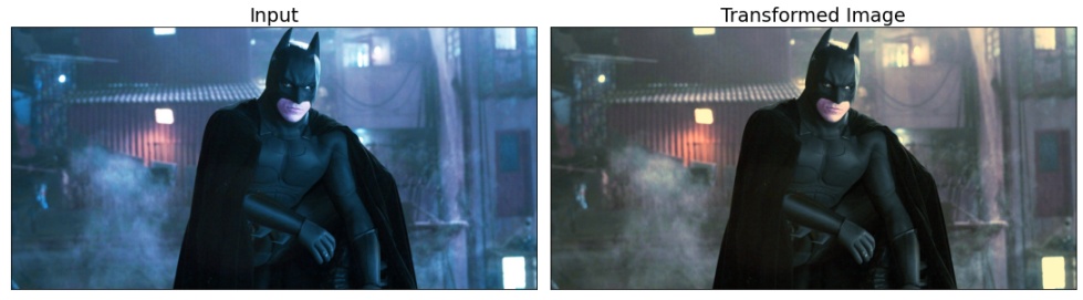
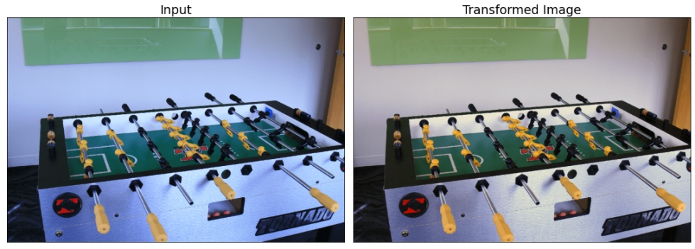
As chromatic adaptation is done with reference white point, the transformed images contain improved white color ranges and other colors are transformed based on illumination transform obtained by white point transform.

As illumination estimation is a crucial step, we can improve results further by applying other illumination estimation methods and images with uniform color objects.

ColorChecker

ColorChecker is a color checker chart containing multiple color squares or rectangles in a grid. ColorChecker chart contains a range of spectral reflectance color patches that represents natural object colors like human skin, leaves, flowers, sky, etc. These color patches on a whole represent all possible intensity ranges that are suitable for many uniform illumination conditions.

ColorChecker charts are used in photography while shooting images/videos under varying illumination conditions. Multiple scenes are shot under varying lighting conditions placing ColorChecker chart in the scene, and later based on the color patches illumination, images are adjusted to destination illuminant. This process is called color grading and it involves several steps including chromatic adaptation.

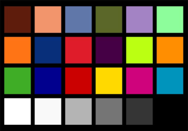Macbeth ColorChecker chart

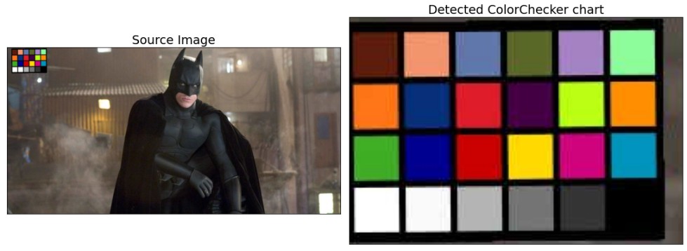
As the color checker chart contains uniform color ranges, we can use this chart to estimate the illuminant of an image. We can detect ColorChecker chart in an image using OpenCV using OpenCV-Contrib module mcc (Macbeth ColorChecker).

1def get_colorchecker_coord(img):
2    # initialize CCDetector object
3    checker_detector = cv2.mcc.CCheckerDetector_create()
4    # detect classic Macbeth 24 color grid chart
5    has_chart = checker_detector.process(img, cv2.mcc.MCC24, 1)
6    # if any chart present
7    if has_chart:
8        # ColorChecker chart coordinates
9        # order - (tl, tr, br, bl)
10        box = checker_detector.getListColorChecker()[0].getBox()
11        min_x = int(min(box[0][0], box[3][0]))
12        max_x = int(max(box[1][0], box[2][0]))
13        min_y = int(min(box[0][1], box[1][1]))
14        max_y = int(max(box[2][1], box[3][1]))
15        coord = [(min_x, min_y), (max_x, max_y)]
16        return [True, coord]
17    else:
18        return [False, []]
19

The above function returns rectangle coordinates (top-left, bottom-right) for ColorChecker chart if present in an image.

We extract ColorChecker from an image and estimate illuminant for only that extracted color chart as it contains uniform color ranges that give a good estimation of illuminant than the whole image.

1src_white_point = np.array([1.0, 1.0, 1.0])
2has_chart, coord = get_colorchecker_coord(img)
3if has_chart:
4    src_white_point = get_gray_world_illuminant(r_img[coord[0][1]: coord[1][1], coord[0][0]: coord[1][0]])
5else:
6    src_white_point = get_gray_world_illuminant(r_img)
7

Chromatic adaptation of the above image with illuminant obtained from cropped ColorChecker chart is

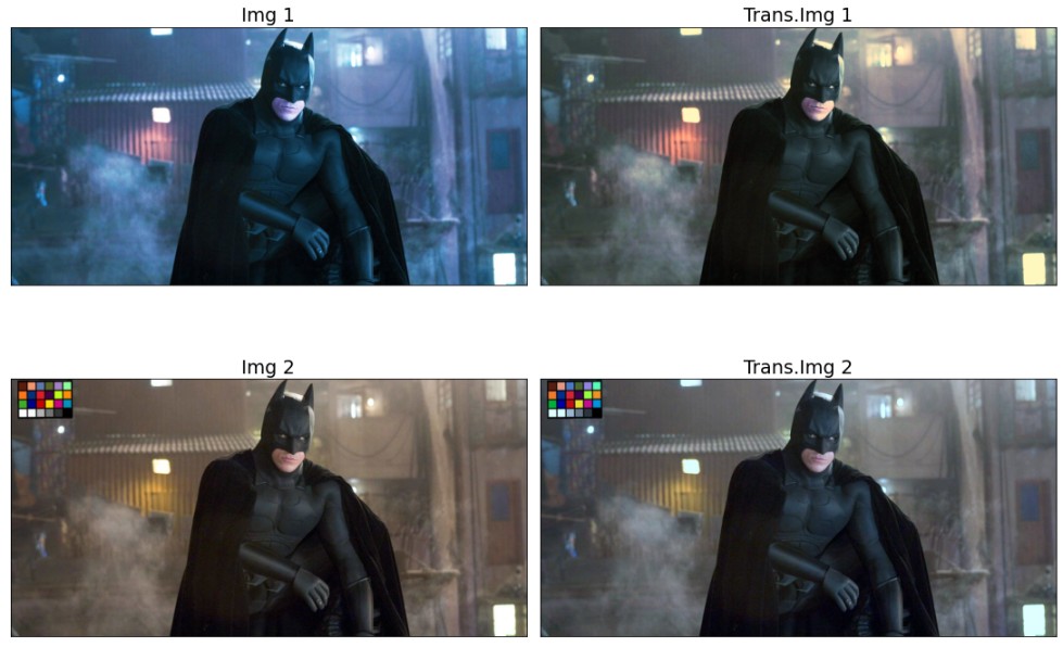
Some regions and color ranges of transformed images of Img 1 and Img 2 are close to each other because we have applied the same destination illuminant for both images and this gives the conclusion that chromatic adaptation works to transform images from one illuminant to another.

We can improve transformation further with better illumination estimation models (both uniform and non-uniform) and compare various chromatic adaptation transform models.

References

• https://www.cell.com/current-biology/pdf/S0960-9822(07)01839-8.pdf
• http://www.marcelpatek.com/color.html
• http://www.brucelindbloom.com/index.html?Eqn_ChromAdapt.html
• https://web.stanford.edu/~sujason/ColorBalancing/adaptation.html
• https://in.mathworks.com/help/images/color.html
• https://in.mathworks.com/matlabcentral/fileexchange/66682-chromadapt-adjust-color-balance-of-rgb-image-with-chromatic