Published on: Mar 23, 2022

Image Enhancement using Retinex Algorithms

In the previous blog Retinex theory of Color Vision, we discussed the theory behind the Retinex model and other studies related to the human visual system of color constancy explained by the Retinex. Even though Retinex failed to accurately define the human color constancy, over the years the Retinex has been modified and used in many image processing applications mainly image color/contrast enhancement, dynamic image compression, shadow removal, and color balancing. In this blog, we apply the Retinex model and its modification algorithms to enhance the low-light color images.

Types of Retinex

Based on the approach of computing the lightness of an image, Retinex algorithms are broadly categorized into four types as shown in the following image.

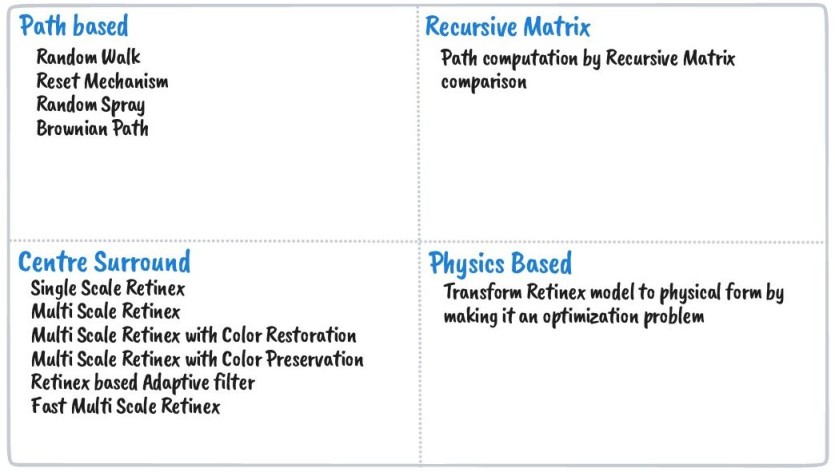
Among the above four types, Center Surround Retinex algorithms are widely used in image processing for image enhancement. In this blog, we discuss applying the following four algorithms from the center-surround category

• Single-Scale Retinex
• Multi-Scale Retinex
• Multi-Scale Retinex with Color Restoration
• Multi-Scale Retinex with Color Preservation

Retinex model and Lightness computation

In the previous blog about Retinex theory, we derived an equation that, the color of an image/scene that we perceive is equal to the illumination on the scene product the reflectance of the scene. When we formulate the previous statement in equation form, that gives

where I is the retinex image, r is the reflectance of the surface, and S is the illumination on the surface. And the lightness of an image, which is computed in our visual system (Retina + Cortex) is computed by reflectance and illumination. If we assume illumination is uniform or smooth, then lightness depends only on reflectance value at a given position.

With this assumption, Land and McCann tried to compute the relative reflectance of an image to estimate the relative lightness of the scene. First, they proposed an algorithm that involves random paths and relative ratios to compute lightness. But that algorithm accuracy highly depends on the number of paths taken, and, it takes so much time to compute the number of paths increases. So, Land published another method to calculate the lightness of a pixel in which the lightness of a pixel is the ratio between the value of a pixel and the average of the surrounding pixels considering the density of these surrounding pixels to have density proportional to the inverse of the square distance.

where $L_{(x,y)}$ is lightness of image at pixel position $(x,y)$, and $F_{(x,y)}*I_{(x,y)}$ is the average of the surrounding pixels at $(x,y)$ given by the center surround function $F_{(x,y)}$.

As the retinex image is equal to the reflectance of the scene under no effect of illumination, the retinex image (R) is approximately equal to the relative lightness. That gives

Single Scale Retinex

Single-scale retinex (SSR) is defined as the difference between the image at a given pixel (x,y) and the center-surround average of that pixel (x,y).

The calculation of the above surrounding pixels average is equal to the inverse square spatial function for a given pixel. And we can use any high pass filter to calculate the surrounding average (Ex. Gaussian distribution) that satisfies the above conditions.

If we consider Gaussian function ($G_{\sigma}$) as center-surround function, then retinex image for each i-th channel in an image is,

That is the Single-scale retinex of an image is estimated by taking the logarithm difference of image and point-surround filter of the image at position (x,y). The operation $(G_{\sigma}*I_i)(x,y)$ is nothing but gaussian blur of an image with given scale ($\sigma$). The implementation in python is pretty straight-forward as

1import numpy as np
2import cv2
3
4def get_ksize(sigma):
5    # opencv calculates ksize from sigma as
6    # sigma = 0.3*((ksize-1)*0.5 - 1) + 0.8
7    # then ksize from sigma is
8    # ksize = ((sigma - 0.8)/0.15) + 2.0
9
10    return int(((sigma - 0.8)/0.15) + 2.0)
11
12def get_gaussian_blur(img, ksize=0, sigma=5):
13    # if ksize == 0, then compute ksize from sigma
14    if ksize == 0:
15        ksize = get_ksize(sigma)
16
17    # Gaussian 2D-kernel can be seperable into 2-orthogonal vectors
18    # then compute full kernel by taking outer product or simply mul(V, V.T)
19    sep_k = cv2.getGaussianKernel(ksize, sigma)
20
21    # if ksize >= 11, then convolution is computed by applying fourier transform
22    return cv2.filter2D(img, -1, np.outer(sep_k, sep_k))
23
24def ssr(img, sigma):
25    # Single-scale retinex of an image
26    # SSR(x, y) = log(I(x, y)) - log(I(x, y)*F(x, y))
27    # F = surrounding function, here Gaussian
28
29    return np.log10(img) - np.log10(get_gaussian_blur(img, ksize=0, sigma=sigma) + 1.0)
30

The function ssr() takes arguments of an image, for which retinex has to be estimated, and sigma value for Gaussian distribution. It returns the single-scale retinex image by subtracting the image and gaussian blur of an image.

get_gaussian_blur() gives Gaussian blur of an image. In this function, we are not using normal cv2.GaussianBlur() method but calculating Gaussian blur using cv2.filter2D() using linear seperability of Gaussian distribution kernels. The reason is, cv2.GaussianBlur() is too slow for large kernels. But cv2.filter2D() applies filter to an image using fast-Fourier transform if kernel size (ksize) > 11. fast Fourier transform computes the convolution in a very few milliseconds than the traditional convolution that takes days or even years to complete.

As OpenCV implementation of fast-Fourier transform is faster than NumPy implementation, we proceed with OpenCV default Fourier transform implementations instead of NumPy or SciPy.

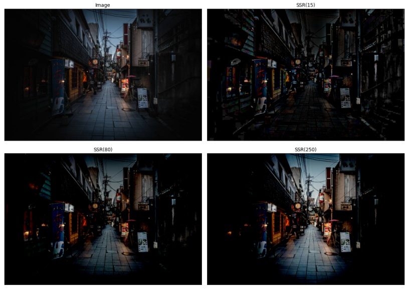
In the above image, for SSR with $\sigma$=15, the output image has some corner areas enhanced but the color is not preserved and it all looks very dark and gray. In SSR(80) image, there has been some improvement in contrast enhancement than SSR(15), but the corner regions became dark and the overall picture looks gloomy. And finally, in SSR(250) image, a significant contrast improvement is done compared to both SSR(15) and SSR(80), but the corner regions became darker than the original image, and only the center region has been enhanced.

It is great that with simple subtraction of image and gaussian image we have enhanced parts of an image to look better but still not a good solution for overall performance. And results are different for different scale values and it is hard to select any single scale value that gives the best results as enhancement purely depends on the nature of the image.

Multi Scale Retinex

As the choice of $\sigma$ varies for different images for good results and different scale values enhance different parts of an image, we can combine SSR of different scales and give weightage for each scale and take a summation of all weighted-SSR images. This method is called Multi-scale retinex (MSR) of an image and it is defined as the weighted average of n single-scale retinex images for different $\sigma$ values.

As the output $MSR_i{(x,y)}$ image might contain negative real values and the range of values is not suitable for image representaion i.e not in range [0-255], normalize the MSR output for range [0-255] given by the following equation

where for channel $i$, $MSR_i{(x,y)}$ is the pixel value at position $(x,y)$, $\min(MSR_i)$ is minimum value of the channel, and $\max(MSR_i)$ is maximum value of the channel

So, Multi-scale retinex is calculated by taking single-scale retinex for different scales and it is computed by the following function

1def msr(img, sigma_scales=[15, 80, 250]):
2    # Multi-scale retinex of an image
3    # MSR(x,y) = sum(weight[i]*SSR(x,y, scale[i])), i = {1..n} scales
4
5    msr = np.zeros(img.shape)
6    # for each sigma scale compute SSR
7    for sigma in sigma_scales:
8        msr += ssr(img, sigma)
9
10    # divide MSR by weights of each scale
11    # here we use equal weights
12    msr = msr / len(sigma_scales)
13
14    # computed MSR could be in range [-k, +l], k and l could be any real value
15    # so normalize the MSR image values in range [0, 255]
16    msr = cv2.normalize(msr, None, 0, 255, cv2.NORM_MINMAX, dtype=cv2.CV_8UC3)
17
18    return msr
19

We give default sigma scale values as [15, 80, 250] with equal weights which preserve high, middle, and low frequencies of an image respectively. msr() computes the MSR of an image by calculating SSR for each $\sigma$ scale. In the end, normalization of the MSR output is done because the computed values could be negative real values and not in a suitable range [0-255] for image representation.

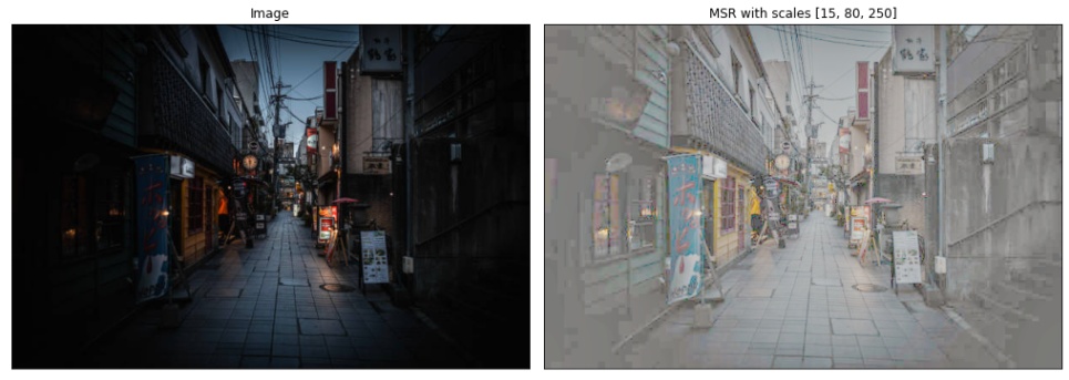
The MSR image for the above input image with scales [15, 80, 250] has many areas enhanced especially in the corner regions which are darker in the input image given by SSR(15). And the retinex output has contrast separation comparatively better than the input image added by SSR(80) and SSR(250), but the output image has an overall gray appeal.

The output MSR image is looking gray because retinex assumes the scene as in Gray world where the average of all colors in the scene is close to gray color. If this assumption is failed in the input image, that is if there are colors that dominate the scene or some colors may not present, whatever the reason could be if the overall color average is not close to gray, then taking the average of multiple single-scale retinex images with equal weights gives output image with colors less saturated and close to gray color. So, we have to modify the Multi-scale retinex to preserve the color of the image.

Multi Scale Retinex with Color Restoration

As the MSR of an image looks colorless, the Multi-scale retinex output is multiplied with Color-restoration function (CRF) of chromaticity to restore the original colors of the input image approximately. And this method of calculating the Color-restoration function and applying it to Multi-scale retinex output is called Multi-scale retinex with Color Restoration (MSRCR).

where $CRF_i{(x,y)}$ is color restoration vlaue for pixel (x,y) at i-th channel. The color restoration function is defined as

where for i-th channel, at position $(x,y)$, CRF depends on the ratio composition of the pixel at (x,y) for that channel value to the sum of all channel values which is equal to calculating chromaticity coordinates. Chromaticity coordinates are calculated as

where $k$ equals to no. of image channels, $\alpha$ is to control non-linearity, and $\beta$ is to control total gain. The above equation can be written as

To achieve better contrast results, the MSRCR equation is modified to include gain (G) and offset (b) values.

The gain and offset values are introduced to transform the contrast range of the MSRCR image to distribute uniformly and to attenuate tails forming in the histogram graph. But these values are not general and don't work for every image. And to stretch the contrast, the final MSRCR image is contrast stretched using Simplest Color Balance algorithm with a clipping percentage of 1% at both ends.

We use default values suggested by different publishers for the above variables as $\alpha=125, \beta=46, G=192, b=-30$

1def color_balance(img, low_per, high_per):
2    '''Contrast stretch img by histogram equilization with black and white cap'''
3
4    tot_pix = img.shape[1] * img.shape[0]
5    # no.of pixels to black-out and white-out
6    low_count = tot_pix * low_per / 100
7    high_count = tot_pix * (100 - high_per) / 100
8
9    # channels of image
10    ch_list = []
11    if len(img.shape) == 2:
12        ch_list = [img]
13    else:
14        ch_list = cv2.split(img)
15
16    cs_img = []
17    # for each channel, apply contrast-stretch
18    for i in range(len(ch_list)):
19        ch = ch_list[i]
20        # cummulative histogram sum of channel
21        cum_hist_sum = np.cumsum(cv2.calcHist([ch], [0], None, [256], (0, 256)))
22
23        # find indices for blacking and whiting out pixels
24        li, hi = np.searchsorted(cum_hist_sum, (low_count, high_count))
25        if (li == hi):
26            cs_img.append(ch)
27            continue
28        # lut with min-max normalization for [0-255] bins
29        lut = np.array([0 if i < li
30                        else (255 if i > hi else round((i - li) / (hi - li) * 255))
31                        for i in np.arange(0, 256)], dtype = 'uint8')
32        # constrast-stretch channel
33        cs_ch = cv2.LUT(ch, lut)
34        cs_img.append(cs_ch)
35
36    if len(cs_img) == 1:
37        return np.squeeze(cs_img)
38    elif len(cs_img) > 1:
39        return cv2.merge(cs_img)
40    return None
41
42def msrcr(img, sigma_scales=[15, 80, 250], alpha=125, beta=46, G=192, b=-30, low_per=1, high_per=1):
43    # Multi-scale retinex with Color Restoration
44    # MSRCR(x,y) = G * [MSR(x,y)*CRF(x,y) - b], G=gain and b=offset
45    # CRF(x,y) = beta*[log(alpha*I(x,y) - log(I'(x,y))]
46    # I'(x,y) = sum(Ic(x,y)), c={0...k-1}, k=no.of channels
47
48    img = img.astype(np.float64) + 1.0
49    # Multi-scale retinex and don't normalize the output
50    msr_img = msr(img, sigma_scales, apply_normalization=False)
51    # Color-restoration function
52    crf = beta * (np.log10(alpha * img) - np.log10(np.sum(img, axis=2, keepdims=True)))
53    # MSRCR
54    msrcr = G * (msr_img*crf - b)
55    # normalize MSRCR
56    msrcr = cv2.normalize(msrcr, None, 0, 255, cv2.NORM_MINMAX, dtype=cv2.CV_8UC3)
57    # color balance the final MSRCR to flat the histogram distribution with tails on both sides
58    msrcr = color_balance(msrcr, low_per, high_per)
59
60    return msrcr
61

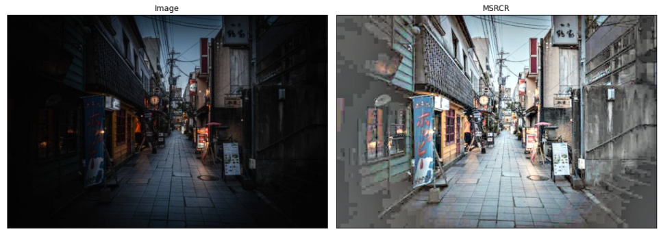
In the above MSRCR output image, the color contrast has been improved compared to Multi-scale retinex. Still, the color contrast is not as close to the original image. With using default values for gain, offset, and others, there might be a chance that some pixels will over-saturate and some will under-saturate. And working around different value settings for different images is not expected behavior from a good enhancement algorithm. The main drawback of this algorithm is to control at least 6 variables which is not a general working method.

Multi Scale Retinex with Color Preservation

In the previous algorithm MSRCR, color restoration was the main issue, and to address that we have introduced many variables and operations. All these calculations are computed directly on each channel value that changes chromaticity coordinates/color composition and the final result is unwanted colors, reversed color order, and sometimes grayish region due to surrounding average. To maintain the chromaticity/color composition as it is and also enhance the color contrast globally on the image, we can apply Multi-scale retinex on intensity image-channel which is just an addition of all image channels divided by the total number of channels.

where $k$ is no. of image channels.

After applying Multi-scale retinex to the intensity image, apply contrast stretch like applied in MSRCR to set the image values in the range [0-255] with uniform distribution of histogram values.

after the MSR, apply the color balance step with a percentage clipping of 1% on both sides.

Finally, preserving the initial chromaticity ratio between each image-channel and intensity image, multiply the ratio with enhance-intensity image channel for each image-channel to get the whole image.

As we are applying retinex enhancement only on intensity-image, each color changes proportional to the ratio between enhance-intensity and normal intensity values. This keeps the relative intensity between surrounding colors locally and globally and gives better results than MSRCR.

1def msrcp(img, sigma_scales=[15, 80, 250], low_per=1, high_per=1):
2    # Multi-scale retinex with Color Preservation
3    # Int(x,y) = sum(Ic(x,y))/3, c={0...k-1}, k=no.of channels
4    # MSR_Int(x,y) = MSR(Int(x,y)), and apply color balance
5    # B(x,y) = MAX_VALUE/max(Ic(x,y))
6    # A(x,y) = max(B(x,y), MSR_Int(x,y)/Int(x,y))
7    # MSRCP = A*I
8
9    # Intensity image (Int)
10    int_img = (np.sum(img, axis=2) / img.shape[2]) + 1.0
11    # Multi-scale retinex of intensity image (MSR)
12    msr_int = msr(int_img, sigma_scales)
13    # color balance of MSR
14    msr_cb = color_balance(msr_int, low_per, high_per)
15
16    # B = MAX/max(Ic)
17    B = 256.0 / (np.max(img, axis=2) + 1.0)
18    # BB = stack(B, MSR/Int)
19    BB = np.array([B, msr_cb/int_img])
20    # A = min(BB)
21    A = np.min(BB, axis=0)
22    # MSRCP = A*I
23    msrcp = np.clip(np.expand_dims(A, 2) * img, 0.0, 255.0)
24
25    return msrcp.astype(np.uint8)
26

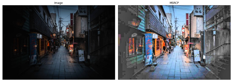
The final MSRCP image above is looking much better than the MSRCR image by preserving relative color intensities in surrounding areas like stand boards have colors enhanced with maintaining relative color ratios between surroundings. The dark regions around the corner are transformed to bright colors but unwanted gray blocks are also upscaled due to a lack of texture information.

Result of other images

The output results for other images are

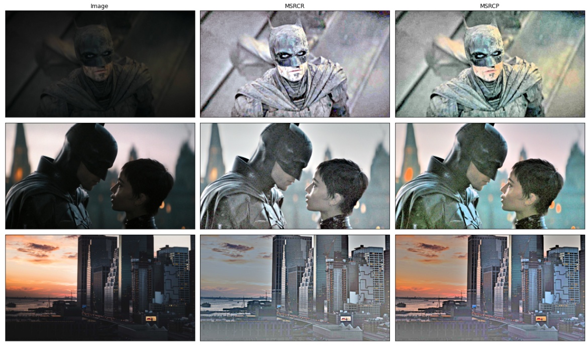
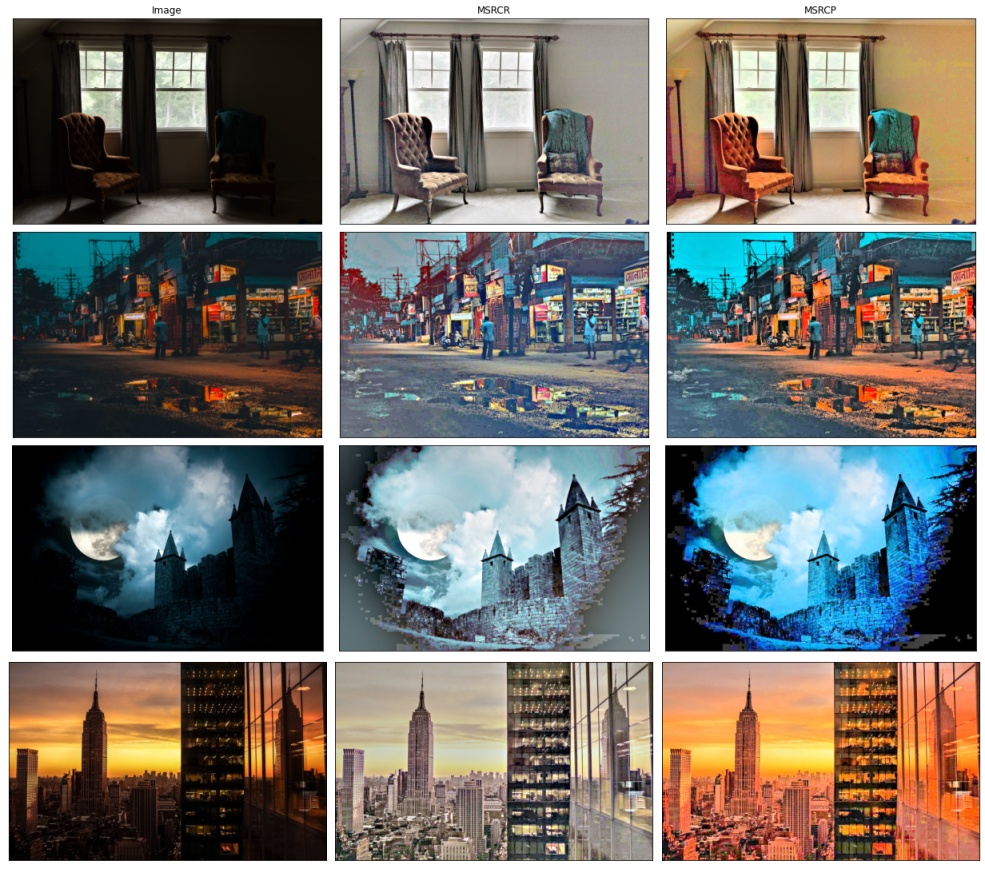
The MSRCP output images are better than MSRCR if the scene has different colors like in images 4th, 5th, and 7th image. Under mono-color illumination like in the 6th image, MSRCP gave a highly saturated blue image while the output from MSRCR looks decent. Choice of the algorithm depends on the scene conditions like illumination, object colors, etc.

The Retinex algorithms presented in the above sections are very basic but gave good results. Most of the super-enhance, image super-resolution, and image-compression models have an underlying model structure based on Retinex. There are other modified Retinex algorithms developed by Gimp, NASA, etc, which give industry-level results. Without training deep-learning models, we can use these Retinex algorithms to implement simple image-enhance filters where we can save resources and time.

References

• Retinex Theory of Color Vision
• Multiscale Retinex